Continual learning aims to learn a series of tasks sequentially without forgetting the knowledge acquired from the previous ones. In this work, we propose the Hessian Aware Low-Rank Perturbation algorithm for continual learning. By modeling the parameter transitions along the sequential tasks with the weight matrix transformation, we propose to apply the low-rank approximation on the task-adaptive parameters in each layer of the neural networks. Specifically, we theoretically demonstrate the quantitative relationship between the Hessian and the proposed low-rank approximation. The approximation ranks are then globally determined according to the marginal increment of the empirical loss estimated by the layer-specific gradient and low-rank approximation error. Furthermore, we control the model capacity by pruning less important parameters to diminish the parameter growth. We conduct extensive experiments on various benchmarks, including a dataset with large-scale tasks, and compare our method against some recent state-of-the-art methods to demonstrate the effectiveness and scalability of our proposed method. Empirical results show that our method performs better on different benchmarks, especially in achieving task order robustness and handling the forgetting issue.

This paper proposed to apply the low rank approximation on the weight transitions in continual learning (CL) and the Hessian information was adopted to determine the preserved ranks.

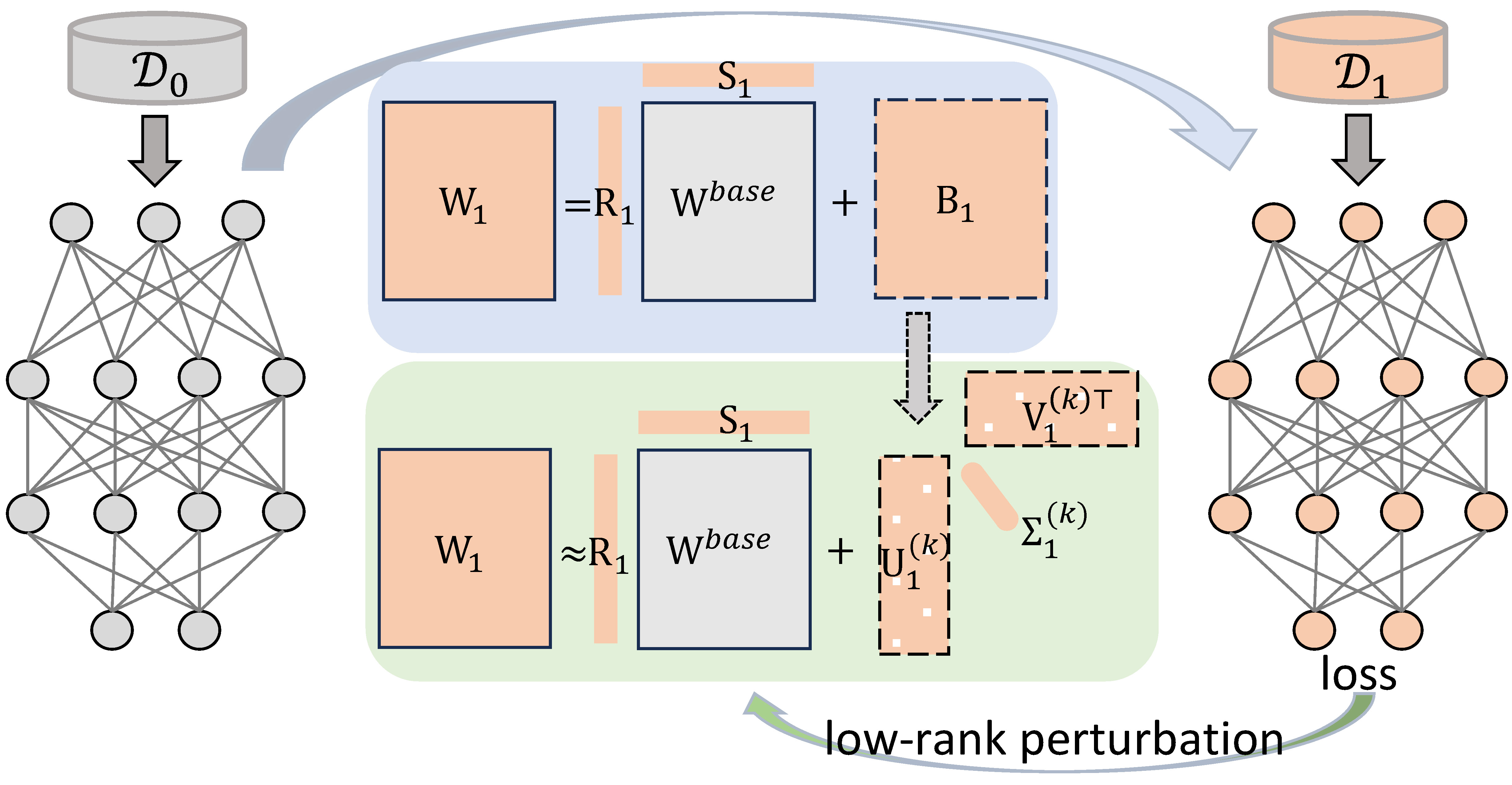
In CL, the model received $T$ tasks in the sequential form \(\{\mathcal{T}_{0}, ..., \mathcal{T}_{T-1}\}\) with datasets \(\{\mathcal{D}_{0}, ..., \mathcal{D}_{T-1}\}\), respectively. We denote the weights in the neural networks as $\mathbf{W}$.

Parameters Transition

In our work, we proposed to model the parameters transition between the tasks as:

\[\mathbf{W}_{t} = \mathbf{R}_{t} \mathbf{W}^{\text{base}} \mathbf{S}_{t} + \mathbf{B}_{t} \tag{1}\]

where

• $\mathbf{W}^{\text{base}}$: the weights obtained on first task \(\mathcal{T}_{0}\) (training process on \(\mathcal{T}_{0}\) is nothing special);
• $\mathbf{W}^{t}$: the weights for successive tasks since \(\mathcal{T}_{1}\) (i.e., $t=1,2,…,T-1$, training process will be introduced later);
• $\mathbf{R}_{t}$= \(\begin{bmatrix} r_{1} & \cdots & 0 \\ \vdots & \ddots & \vdots \\ 0 & \cdots & r_{J} \\ \end{bmatrix}\)

and $\mathbf{S}_{1}$= \(\begin{bmatrix} s_{1} & \cdots & 0 \\ \vdots & \ddots & \vdots \\ 0 & \cdots & s_{I} \\ \end{bmatrix}\) are two (diagonal) scaling matrices:

• $\mathbf{B}_{t}$ is the residual matrix.

Low-Rank Approximation

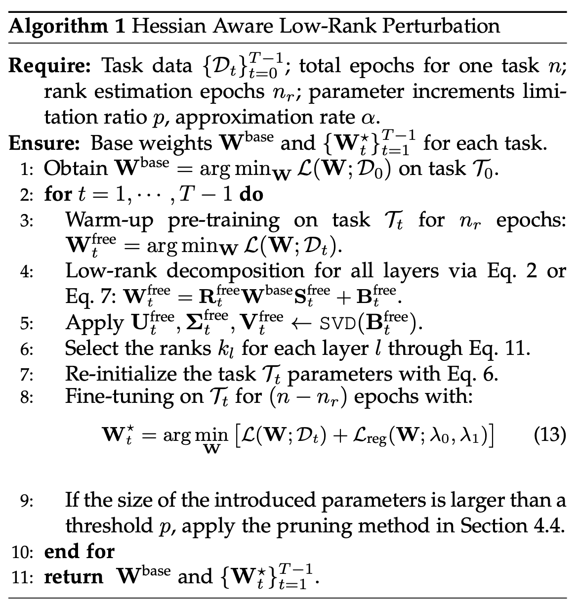
Once a new taks \(\mathcal{T}_{t}\) (with $t=1,2,…,T-1$) comes, we firstly do a warm-up training (e.g., one or two epochs) without any constraints. This process returns the weights as $\mathbf{W}^{\text{free}}_{t}$, a rough estimation FOR $\mathbf{W}^{t}$.

Our objective is to further compress the residual weight $\mathbf{B}^{\text{free}}_t$ via low-rank approximation:

\[\mathbf{U}_{t}^{\text{free}}, \mathbf{\Sigma}_{1}^{\text{free}}, \mathbf{V}_{1}^{\text{free}} \leftarrow \texttt{SVD}(\mathbf{B}_{1}^{\text{free}}) \tag{2}\]

then

\[\mathbf{W}_{t}^{\text{free}} \approx \mathbf{W}_{t}^{(k){\text{free}}} = \mathbf{R}_{t}^{\text{free}} \mathbf{W}^{\text{base}} \mathbf{S}_{t}^{\text{free}} + \mathbf{B}_{t}^{(k){\text{free}}} \tag{3}\]

with

\[\mathbf{B}_{t}^{(k){\text{free}}} = \mathbf{U}_{t}^{(k){\text{free}}} \mathbf{\Sigma}_{t}^{(k){\text{free}}} (\mathbf{V}_{t}^{(k){\text{free}}})^\top \tag{4}\]

Rank Selection by Hessian-Aware Information

Now, here comes the question:

How many ranks $k_l$ should we preserve for each layer $l$ in a neural network?

Firstly, let’s consider how a weight perturbation will affection the loss change within in a neural network:

Theorem 1: Assume that a neural network of \(L\) layers with vectorized weights \((\mathbf{\omega}^{\star}_{1}, \dots, \mathbf{\omega}^{\star}_{L})\) that have converged to local optima, such that the first and second order optimally conditions are satisfied, \emph{i.e.}, the gradient is zero, and the Hessian is positive semi-definite. Suppose a perturbation \(\Delta \mathbf{\omega}^{\star}_{1}\) applied to the first layer weights, then we have the loss change

\[\big|\mathcal{L}(\mathbf{\omega}^{\star}_{1} -\Delta \mathbf{\omega}^{\star}_{1}, \dots, \mathbf{\omega}^{\star}_{L}) - \mathcal{L}(\mathbf{\omega}^{\star}_{1}, \dots, \mathbf{\omega}^{\star}_{L}) \big| \leq \frac{1}{2}\|\mathbf{H}_{1}\|_F \cdot \|\Delta \mathbf{\omega}^{\star}_{1}\|^2_F +o\left(\|\Delta \mathbf{\omega}^{\star}_{1}\|^2_F\right) \tag{6}\]

where \(\mathbf{H}_1=\nabla^2\mathcal{L}(\mathbf{\omega}^{\star}_1)\) is the Hessian matrix at only the variables of the first layer weights. It holds for any layer \(l\).

Approximating \(\mathbf{W}_{t}^{\text{free}}\) by \(\mathbf{W}_{t}^{(k)\text{free}}\) can be considered as a perturbation \(\Delta\mathbf{W}_{t}^{\text{free}}\) on the original parameters:

\[\Delta \mathbf{W}_{t}^{\text{free}} = \mathbf{W}_{t}^{\text{free}} - \mathbf{W}_{t}^{(k){\text{free}}} \tag{7}\] \[\|\Delta \mathbf{W}_{t}^{\text{free}}\|_{F} = \|\mathbf{W}_{t}^{\text{free}} - \mathbf{W}_{t}^{(k){\text{free}}}\|_{F} = \sqrt{\sum_{i=k+1}^{r}\sigma_i^2} \tag{8}\]

where \(\sigma_i\) is the \(i\)-th singular value in \(\mathbf{\Sigma}_{t}^{\text{free}}\), indicating the \(i\)-th rank.

By applying Theorem 1 to the above low rank approximation, we have

\[\left|\mathcal{L}(\mathbf{W}_1^{(k){\text{free}}}) - \mathcal{L}(\mathbf{W}_1^{\text{free}}) \right| \leq \frac{1}{2}\|\mathbf{H}_1\|_F \cdot \left(\sum_{i=k+1}^{r}\sigma_{i}^2\right) +o\left(\sum_{i=k+1}^{r}\sigma_{i}^2\right) \tag{9}\]

Eq.(9) indicates that:

• we need to preserve more ranks (i.e., preserve ranks \(\{1,2,\cdots, k\}\), or discard less ranks \(\{k+1,\cdots, r\}\) in other words) to achieve smaller approximation errors (i.e., controlled by a tighter upper-bound controlled by the first term in RHS in Eq.(9)).
• the contribution of a certain rank $k$ in the $l$-th layer can be measured by

\[\|\mathbf{H}_{l}\|_F \sigma_{l, k}^{2} \tag{10}\]

According to the previous studies, the Hessian matrix \(\mathbf{H}_l\) can be approximated by the empirical negative Fisher information, i.e., the outer product of the gradient vector for the layer weights. So \(\|\mathbf{H}_l\|_{F}\) can be approximated by \(\|\mathbf{g}_{l}\|_F^2\), where \(\mathbf{g}_{l} = \frac{\partial\mathcal{L}}{\partial \mathbf{W}_l}\|_{\mathbf{W}_{l}=\mathbf{W}_{l}^{\text{free}}}\).

Finally, we can quantitatively measure the contribution of the loss of adding a marginal rank $k$ for a particular layer $l$ by

\(\| \mathbf{g}_l \|_2^2 \sigma_{l,k}^2 \tag{11}\).

Based on the above results, we proposed to select the ranks by measure the overall contribution ratio. For a given approximation rate $\alpha$ (e.g., 0.9), we can choose the minimum rank $k_l$ (with $k_l\leq r_l$ where $r_l$ is the total rank of the layer $l$) for each layer $l=1,…,L$ such that the accumulated contribution of preserved ranks can surpass \(\alpha\cdot 100\%\) of the total contribution from all ranks, i.e., by solving the following problem:

\[\min_{k_1,...,k_{L}} \quad \sum_{l=1}^{L} \sum_{i=1}^{k_l} \| \mathbf{g}_l \|_2^2 \sigma_{l,i}^2\\ \text{s.t.} \sum_{l=1}^{L} \sum_{i=1}^{k_l} \| \mathbf{g}_l \|_2^2 \sigma_{l,i}^2 \geq \alpha \cdot \left(\sum_{l=1}^{L} \sum_{i=1}^{r_l} \| \mathbf{g}_l \|_2^2 \sigma_{l,i}^2 \right) \tag{12}\]

The selected ranks are used to re-initialize the model weights for completing the remaining training process.

Remark: The above illustration gives an example of the above rank selection process for $L=3$:

• Top$\rightarrow$Left: Apply Singular Value Decomposition $\texttt{SVD}(\cdot)$ on the parameters obtained by the warm-up training on a new task.
• Left$\rightarrow$Bottom: After obtaining the singular values $\sigma_{k,l}$ for each rank and the gradient $\mathbf{g}_l$ for each layer $l$, we can sort the values of \(\| \mathbf{g}_l \|_2^2 \cdot \sigma_{l,k}^2\) for all ranks within all layers by decending order.
• Bottom$\rightarrow$Right: We determine the ranks $k_l$ for each layer $l$ by making a truncation such that the accumulated contribution properly surpasses the overall contribution by a proportion $\alpha \cdot 100\%$. We can see that we preserve the number of ranks $k_1=2, k_2=3, k_3=2$ for each layer in this example, respectively.
• Right$\rightarrow$Top: The model weights are re-initialized with the approximated parameters \(\mathbf{U}_{t}^{(k_l){\text{free}}}, \mathbf{\Sigma}_{t}^{(k_l){\text{free}}}, \mathbf{V}_{t}^{(k_l){\text{free}}}\) before finishing the remaining fine-turning epochs.

Summary

The overall algorithm description of our proposed HALRP is:

Experiments

We conducted extensive experiments on CIFAR100, P-MNIST, Five-dataset, Omniglot-Rotation, TinyImageNet with different backbones to demonstrate the effectiveness of our methods. The empirical results showed that our method achieved a better trade-off regarding avoiding forgetting issue, controlling model size increment, robustness on task orders, and efficiency. More details can be found in our paper.